

This section explains the different elements and steps that a risk assessment for heavy rain induced flooding might consist of. It shows different methodological approaches for these steps and describes their pros and cons as well as demands for data and resources. In-depth knowledge and experiences from implementing different methods in different areas is provided via our lessons-learnt as well as scientific reports from the RAINMAN project.

SOURCE ANALYSIS
The source analysis gives answers to questions dealing with the generation of surface runoff depending on the precipitation event and the processes happening on the surface such as infiltration.
PATHWAY ANALYSIS
The pathway analysis describes the processes of surface runoff concentration and runoff routing, i.e. the flow dynamics of the water. It gives answers to questions such as: Which flow pathways does the water take? At what level is the water flowing or ponding? What is the distribution of flow velocities?
After the rainwater has reached the surface it is transformed to surface water depending on the runoff generation process and the influence of the surface material. The water on the surface follows the slope of the terrain and concentrates in areas where water from different source regions meets. The area that belongs to a point where water can come from is called its catchment. The bigger the catchment area of a point, the higher is the potential amount of water that might reach this point and a high amount of water typically translates to water depth. Slope or steepness of the terrain surface has a strong influence on flow velocity as well as the roughness of the surface, e.g. smooth and “fast” concrete road vs. rough and “slow” dense shrubs. Pathways of concentrated runoff can be known rivers and creeks as well as unknown or barely visible linear depressions that have not been observed as waterways in the past. Especially in flat areas local depressions can fill up and form temporary ponds, a process also known as “ponding”.
Approaches for a pathway analysis can be flow pathways/runoff accumulation methods as well as the computer-based modelling of the flow of water based on physical principles (hydrodynamic simulation methods). Details about the potentials and limitations of these approaches can be found below.
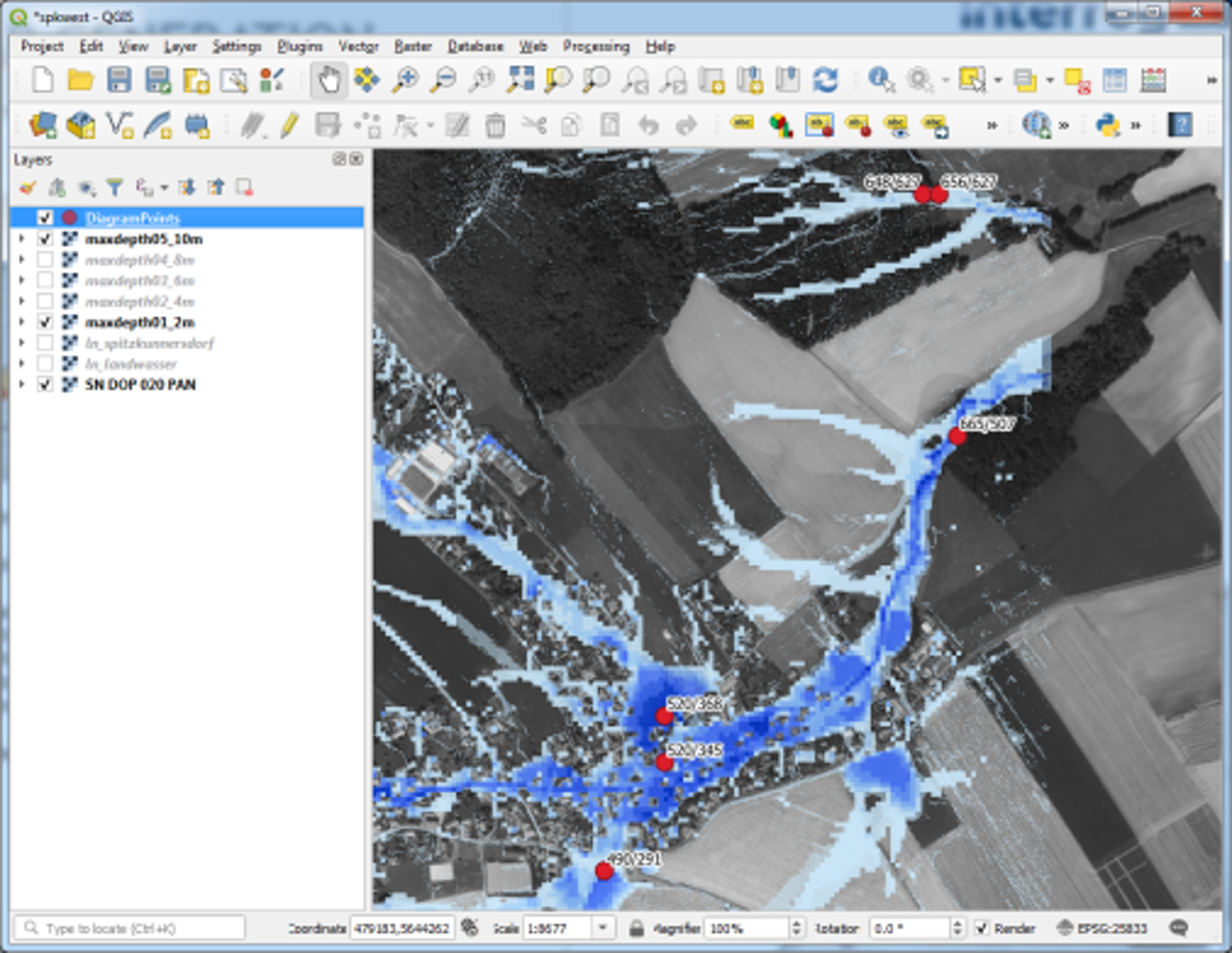
Computer-based modelling of the flow of water. Picture: Axel Sauer, IöR, and GeoSN, dl-de/by-2-0

Local depression has filled up with water (ponding). Picture: Municipality of Leutersdorf (district of Spitzkunnersdorf)

RECEPTOR ANALYSIS
The receptor analysis identifies/maps and characterises subjects and objects that might be harmed or damaged by the flood water.
CONSEQUENCE ANALYSIS
The consequence analysis describes the processes that cause harm and damage to the receptors, e.g. drowning, wetting of building construction elements, erosion of street paving etc.

Picture: Axel Sauer, IöR, and GeoSN, dl-de/by-2-0

Picture: Axel Sauer, IöR, and GeoSN, dl-de/by-2-0
Picture: Axel Sauer, IöR, and GeoSN, dl-de/by-2-0

Picture: Axel Sauer, IöR, and GeoSN, dl-de/by-2-0
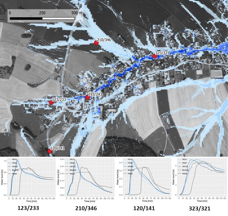
The following map shows the inundation simulated with the 2D hydrodynamic flow model HiPIMS for a subset of the Spitzkunnersdorf (Germany, Saxony) study region and the location of sample points where time series of water levels have been mapped. Five different rainfall inputs can be compared: Three synthetic storms based on the Euler II method with return probabilities of 1 in 10 years (HN10), 1 in 30 years (HN30) and 1 in 100 years (HN100) as well as a so-called block rain (Block54) and the radar precipitation measurement of an observed event (radar). The Euler rains and the block rain are not spatially differentiated and put a homogenous rain field on the catchment. The Euler rains are differentiated over time in contrast to the continuous intensity block rain. The radar rain shows the dynamics in space and time of a real precipitation event.
Picture: Axel Sauer, IöR, and GeoSN, dl-de/by-2-0
Based on their synthetic nature the water level curves of the Euler rains are quite similar regarding their shape. In the upper parts of the catchment the runoff reaction is fast with peak water levels after 20 minutes, in lower parts between 30 and 40 minutes. The rising part of the hydrograph is nearly identical for all rains with a temporal shift of the observed rain due to a different starting time with a longer phase of very low intensities. In this catchment, the peak water levels differ not so much between the different Euler rain return probabilities. In comparison to them the block rain results in substantially lower water levels that stay on a constant level during the precipitation lasts after reaching the peak level. At the downstream point with a deep and narrow riverbed, the resulting water levels are quite close together.
Conclusions
- The rainfall input has a major influence on flow dynamics and water levels.
- It should be stressed that natural precipitation events are highly dynamic and diverse in terms of duration, intensity distribution over time as well as movement directions in space.
- In order to be prepared for probable precipitation events, it is important to simulate a wide variety of rainfall events regarding temporal and spatial patterns and to present alternative maps.
In the following graphics you see the effects of different roughness values on the water levels in the course of time for selected points based on a 1 in 100 years Euler II synthetic precipitation. The Gauckler-Manning-Strickler surface roughness value is for the whole area varied between values of 0.01 and 0.1 in 0.01 steps. The lowest value stands for a very smooth surface such as fine concrete and the highest value for a very rough surface such as a river bed with big boulders or dense shrubs. The GMS value influences the flow velocities and has effects on the water levels and their spatial and temporal distribution.
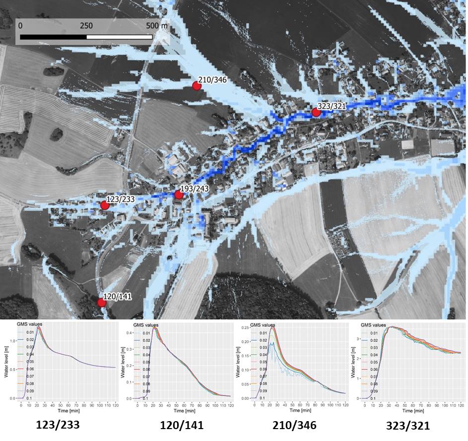
Picture: Axel Sauer, IöR, and GeoSN, dl-de/by-2-0
For this rainfall scenario and the given catchment characteristics the effects of the different GMS roughness values on the dynamics of the water levels for the selected points are relatively small. The lower roughness values are associated with lower water levels and a slightly steeper rise and earlier peak time due to higher flow velocities. It has to be kept in mind that the flow velocities as an important impact indicator can vary substantially more than the water levels.
Conclusions